B7 - boundary conditions
types of boundary conditions
- dirichlet boundary conditions: fixed boundary value, eg:
- von neumann boundary conditions: zero or fixed gradient, eg:
or - periodic boundary conditions on
domain of length, , such that
von neumann BC: 2nd derivative
- evaluating a second derivative for von neumann BC in space at a left boundary,
- the taylor expansion:
- applying
- therefore, the second derivative at
can be expressed as:
- translating this into finite difference expressions:
- von neumann BC using central finite difference scheme:
- therefore:
- this is equivalent to the expression obtained from taylor expansion
boundary value problem
- considering a steady state of 1D heat equation with a source
- steady state:
- finite difference representation:
- the solution at grid point
is coupled to solution at points - writing this set of coupled linear equations using matrix notation:
-
each row of matrix
numbers the equation of a particular grid point -
a column is equivalent to a coupling to the temperature at another grid point
-
the general equation for an arbitrary point
on the grid is:
- approach 1: the domain is discretised by
points with boundaries at and , where
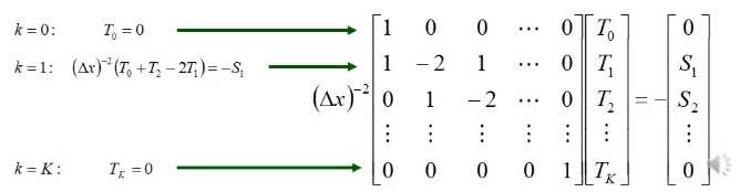
image: B Hnat, lecture notes
- approach 2: the domain is discretised by
points, with boundaries at 'ghost' points, and , with dirichlet BCs: , using which the equations for 'real' grid pints are simplified
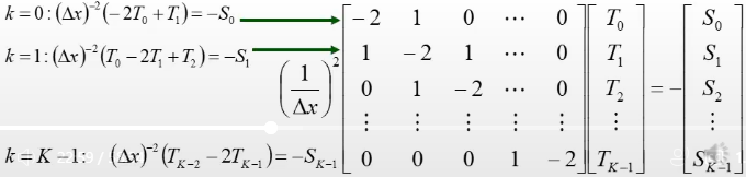
image: B Hnat, lecture notes
- the matrix is sparse (many 0's) and banded (non-zero elements near the diagonal), which can be easily inverted
- only the non-zero elements are needed for matrix inversion, and only these should be stored in the memory
- once solution is found, the original matrix is needed to match the value to a correct grid point
- this requires a formula that gives a row number of a non-zero element for a given column,
- suppose a reduced matrix,
, which contains only the non-zero elements, such that:
is a constant added to assure that the row index is always , which is equal to the number of non-empty bands above/below the diagonal
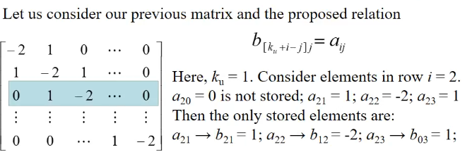
image: B Hnat, lecture notes
- note: arrays are always stored in 1D, so a 2D array,
b[i][j]in C is translated to a single index of an element in a memory block

image: B Hnat, lecture notes
x2 - code for transforming indices
periodic boundaries
- considering a steady state of 1D heat equation:
- the periodic
domain has a length , such that any solution satisfies: and - representing the function at
grid points: , - the periodic boundary implies that:
- the second derivative at the boundary can then be evaluated as:
- at the left boundary:
- at the right boundary:
- this is a matrix problem with
equations and unknowns
- the matrix is sparse, but not banded due to the ones outside the near-diagonal band
- this can be converted into a banded matric by changing the indices of the unknowns
matrix folding
- thinking of it as folding of
domain, so the ends of the domain are at two neighbouring points
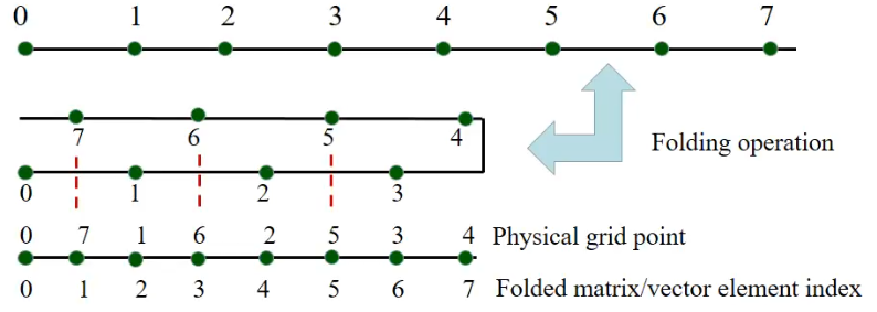
image: B Hnat, lecture notes
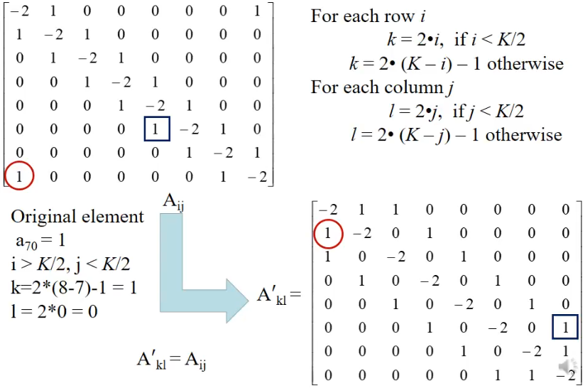
image: B Hnat, lecture notes
- constructing an indexing function that converts between physical locations on the grid and the index of the folded matrix such that for
, the physical location indexed by , there is the matrix element index
-
then:
, and -
the benefits of folding:
- the new matrix,
, does not have entries far from the diagonal - the time to invert a matric scales as
for a full matrix, but for a banded matrix with -elements band
- the new matrix,
-
so
is solved, and is reordered each time the physical grid based is needed -
the indexing function
is used each time the matrix/vector is accessed explicitly